Introduction
In the previous minilab we had a look at how varying the extent of the exponential diffusive overshoot region changes the asymptotic period spacing of dipole ($\ell=1$) modes, $\Pi_{\ell=1}$. An even better option for studying CBM is using the individual g-mode oscillation periods of the stars, and study the changes in the morphology of their period spacing patterns. Such patterns are constructed by calculating the period differences $\Delta P$ between modes of the same degree $\ell$ and azimuthal order $m$ and consecutive radial orders $n$, and then plotting these differences as a function of the oscillation periods. For a chemically homogeneous, non-rotating star we expect these patterns to be homogenous as
\begin{equation} \Delta P \approx P_{2} - P_{1} \approx P_{3} - P_{2} \approx \dots \approx P_{n} - P_{n-1} \approx \frac{\Pi_0}{\sqrt{\ell (\ell +1)}}. \end{equation}
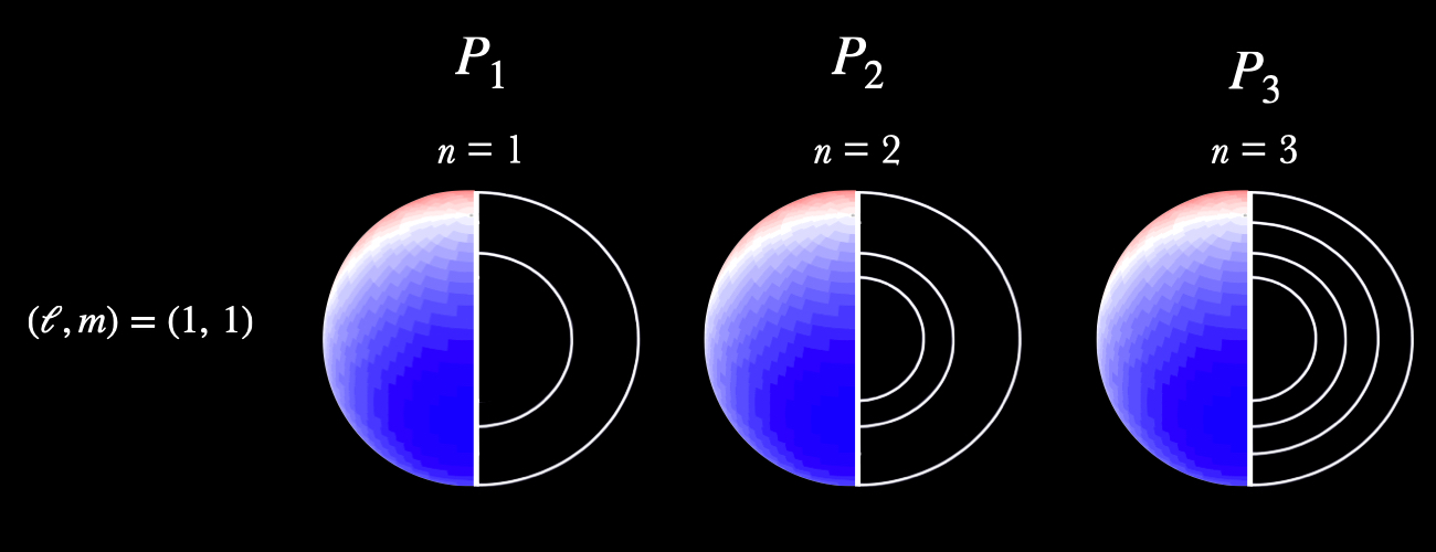
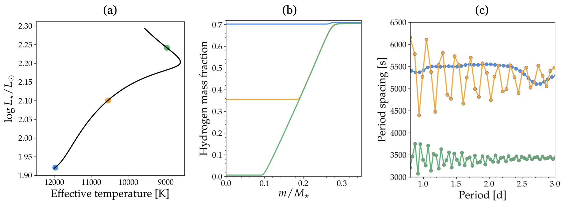
As the star evolves on the main-sequence and consumes hydrogen in its core, the chemical profile of the star is no longer homogenous. Instead a chemical gradient is developed as the convective core contracts during the main-sequence evolution, which traps the oscillations and gives rise to dips in the period spacing pattern as demonstrated in the figure below.
As internal mixing changes this gradient, it likewise results in changes in the morphology of the period spacing pattern. In this minilab we are going to study these changes to the patterns from exponential diffusive overshooting for a terminal age main-sequence $4\,{\rm M}_\odot$ SPB star. In order to calculate the stellar oscillations, we are going to use the stellar oscillation code GYRE which is included as part of the MESA installation.
Aims
MESA + GYRE aims: In this MESA lab you will learn how to run GYRE outside of MESA, what additional parameters are needed in your MESA inlist to generate files needed as input in GYRE, and how to construct a GYRE inlist.
Science aims: Investigating what effect convective boundary mixing has on period spacing patterns of SPB stars.
Minilab 2
Warning! These MESA labs have been put together with both low time and spatial resolution for the sake of having the models be completed within a sensible timeframe for the summer school. Before any of these steps or result can be used in any type of actual science case, carrying out a convergence study is crucial!
Minilab 1 solution: download
Minilab 2 solution: download
For the TAs: Additional instructions for plotting period spacing patterns are available at the bottom of the home page. We expect you to be in charge of plotting these patterns to avoid having the students spend time on trying to get the provided scripts to work. Should they have extra time available, however, they are more than welcome to try out the scripts themselves as well.
The first step of this minilab is making sure that we can run GYRE as a standalone module outside of MESA. In order to be able to do so, we have to set the path to the GYRE directory in your shell-startup file, just like how you had to do so when installing MESA. Depending on your operating system this is likely to either $HOME/.bashrc or $HOME/.zshrc, but you can also check this using the command:
echo $0
The GYRE directory that has to be set is $MESA_DIR/gyre/gyre. So as an example, this is what my $HOME/.zshrc file looks like when the path to GYRE has been set correctly:
export OMP_NUM_THREADS=4

export MESA_DIR=/Users/mped4857/Software/MESA/mesa-r23.05.1

export MESASDK_ROOT=/Applications/mesasdk
source $MESASDK_ROOT/bin/mesasdk_init.sh

export GYRE_DIR=$MESA_DIR/gyre/gyre
Once the path to GYRE has been set, we need to first source our bash shell-startup file
source $HOME/.zshrc
When initially installing MESA, the GYRE code should also have been compiled automatically. However, if this turns out not to be the case for you (this will become clear once you start trying to run GYRE) then you will have to complete the following two steps in your terminal to compile GYRE using make inside your GYRE directory.
cd $GYRE_DIR
make
If the installation went smoothly, then now we should be able to run GYRE outside of MESA!
Let’s start by creating a new MESA work directory by copying the one we created for Minilab 1. If you were unable to complete Minilab 1, then you can download the solution from here.
cp -r SPB_minilab_1 SPB_minilab_2
cd SPB_minilab_2
./clean && ./mk
Also, delete the current contents of your LOGS directory to avoid confusion with previous models from minilab 1.
Before we run GYRE we have to first tell MESA to output profiles in a format that GYRE can read as input. We can do so by modifying the &controls section of inlist_project. These controls are called controls for output in the MESA documentation.
Task 1
Add the following asteroseismology inlist parameters to &controls:
- Tell
MESAto write the pulsation data along with theMESAprofiles. - Set the pulsation data format to
GYRE.
Hint
The parameters that have to be added are: write_pulse_data_with_profile and pulse_data_format
Task 2
Amongst the people at your table, distribute the following values for the overshooting parameter overshoot_f(1) and use that in your inlist_project: 0.01, 0.02, 0.03, and 0.04. Likewise, change your log_directory parameter LOGS/4Msun_#fov to match the new value of the overshooting parameter. Then run MESA.
Your inlist_project should now look something like this.
When MESA is done running you should see that you now have additional output files in your LOGS/4Msun_#fov directory with a ‘GYRE’ extension, one for each of your MESA output profile#.data files of the format profile#.data.GYRE. It is these profile#.data.GYRE files that we need to use as input for the GYRE computations, where we use GYRE to calculate the associated theoretical oscillations for our profile#.data model. We note that as an alternative, the GSM format is another pulsation data format that is written specifically for GYRE and uses an HDF5-based format instead of the plain-text format that we get by using 'GYRE' for the pulse_data_format parameter in inlist_project.
Just like MESA, GYRE also has an inlist file that we have to either create or modify. Information on how to construct such a file is given on the
GYRE documentation website. Discussions, bugs and feature requests can be found on the GYRE discussion forum. As a starting point, let’s create an empty GYRE input file called gyre.in inside our MESA work directory using your favourite text editor.
nano gyre.in
The setup of the different sections (i.e. namelists) that we need to include in gyre.in is the same as for your MESA inlist_project file, i.e. a section starts with &name and ends with /. As a minimum, we want to include the input model specifications (&model), which oscillation modes to compute (&mode), information on the inner and outer boundary of the model (&osc), which numerical solver to use (&num), how to scan the frequency region of interest (&scan), include an oscillatory weight parameter for the spatial grid (&grid), and what to output (&ad_output and &nad_output). More information on how to set these up is given in the Namelist Input Files section on the GYRE documentation website. In addition to the above-mentioned namelist sections, GYRE also requires the physical constants to be defined in &constants as well as specifying the rotation setup (&rot). We are just going to use the default values for these.
&constants
/

&model
/

&rot
/

&mode
/

&osc
/

&num
/

&scan
/

&grid
/

&ad_output
/

&nad_output
/
Task 3
Create a gyre.in file and include the namelist sections &constants, &model, &rot, &mode, &osc, &num, &scan, &grid, &ad_output, and &nad_output as shown above.
Now that we have included the relevant namelist sections for this MESA lab, we will start by telling GYRE which model (file) it should use for the computations. When doing so, we also need to tell GYRE that this input model is an evolutionary model read from an external file (model_type) that was calculated by MESA (file_format). As a start, lets use profile2.data.GYRE as an input file.
Task 4
In the &model namelist section, include the parameters:
file = './LOGS/4Msun_#fov/profile2.data.GYRE'
model_type = 'EVOL'
file_format = 'MESA'
Make sure you use your chosen value of $f_{\rm ov}$ in place of #. Other possible options for how to set these parameters as well as which additional parameters you can add to the &model section are listed under Stellar Model Parameters.
Next, lets setup the &osc and &num namelist sections.
Task 5
In the &osc namelist section set the outer boundary parameter outer_bound = 'VACUUM' and the inner boundary parameter inner_bound = 'REGULAR'. These determine the outer and inner boundary conditions of the model when calculating the oscillations. In &num tell GYRE to use the 4th-order Gauss-Legendre Magnus solver for initial-value integrations 'MAGNUS_GL4' using the diff_scheme parameter.
Once we have our numerics and model specifications, we now want to tell GYRE which oscillations to compute. We will do so using the two namelist sections &mode and &scan. For this MESA lab we will focus on dipole prograde ($\ell =1, m=1$) modes with radial orders between $-1$ and $-80$. Note that by convention, we use negative radial orders for g-modes and positive radial orders for p-modes. In principle, it doesn’t matter what we are setting $m$ to be as long as we are fulfilling $m = -\ell, \dots, \ell$. This is because we are currently not including rotation in our GYRE computations, so all of the $m = -\ell, \dots, \ell$ modes for the same $\ell$ and $n$ value would have the same frequency. To include rotation, we would have to include additional parameters in the &rot namelist section in our GYRE inlist file as rotation is turned off by default. You will see more on this during the MESA lab sessions on Thursday. For now, we stick to using ($\ell =1, m=1$) as these are the modes most commonly detected in SPB stars.
Task 6
In the &mode namelist section, include the parameters:
l = 1
m = 1
n_pg_min = -80
n_pg_max = -1
The relevant frequency range to consider for g-modes in SPB stars is between $0.05 {\rm d}^{-1}$0.05d-1 and $5 {\rm d}^{-1}$ 5d-1. We will tell GYRE to split this range into 400 bins that are equally spaced in period rather than frequency. This is because the g-modes are approximately equally spaced in period contrary to p-modes that are equally spaced in frequency. Finally, we want the oscillation frequencies to be calculated in the inertial (i.e. observer) frame of reference. For recommendations on how to set up your Frequency Grid you can check out the Understanding Grids section on the GYRE documentation website.
Task 7
In the &scan namelist section, include the parameters:
grid_type = 'INVERSE'
freq_frame = 'INERTIAL'
freq_min = 0.05
freq_max = 5
freq_min_units = 'CYC_PER_DAY'
freq_max_units = 'CYC_PER_DAY'
n_freq = 400
When computing the oscillations we want to make sure that we have a high resolution in the spatial grid where large variations in the displacement perturbation $\xi$ are occurring. We do so by adding three additional parameters to &grid which are described in detail in Spatial Grids section on the GYRE documentation website.
Task 8
In the &grid namelist section, include the parameters:
w_osc = 10
w_exp = 2
w_ctr = 10
Now our last step is to tell GYRE what to output using &ad_output. There are two types of output files to consider: the summary and detail output files. The summary file provides an overview of the GYRE calculations for all considered modes, such as their frequencies, degree $\ell$, and azimuthal order $m$ values, whereas the detail files provide additional information on each one of the calculated modes such as their radial ($\xi_r$) and horizontal ($\xi_h$) displacements as a function of the radius coordinate. You, therefore, get one detail file per calculated mode. In this MESA lab, we are only interested in the summary files.
Task 9
In the &ad_output namelist section, include the parameters:
summary_file = './LOGS/4Msun_#fov/profile2_summary.txt'
summary_file_format = 'TXT'
summary_item_list = 'l,m,n_p,n_g,n_pg,freq'
freq_units = 'CYC_PER_DAY'
Did you notice that we will only be asking GYRE to output the adiabatic solutions (&ad_output) to the oscillation equations? We choose to do so here for a couple of reasons. The first and most important one is because it is faster and for this MESA lab, we are not going to look into which modes are excited which would require us to find the non-adiabatic solutions (&nad_output). The second reason is that we generally observe more modes than what are predicted to be excited by the standard opacity tables in MESA. We note that changing from adiabatic to nonadiabatic calculations will not result in any significant changes to the output oscillation frequencies, but is required in order to determine which modes are predicted to be excited.
If you have done everything correctly, then your gyre.in file should now look something like this
&constants
/

&model
  file = './LOGS/4Msun_0.01fov/profile2.data.GYRE'
  model_type = 'EVOL'
  file_format = 'MESA'
/

&rot
/

&mode
  l = 1
  m = 1
  n_pg_min = -80
  n_pg_max = -1
/

&osc
  outer_bound = 'VACUUM'
  inner_bound = 'REGULAR'
/

&num
  diff_scheme = 'MAGNUS_GL4'
/

&scan
  grid_type = 'INVERSE'
  freq_frame = 'INERTIAL'
  freq_min = 0.05
  freq_max = 5
  freq_min_units = 'CYC_PER_DAY'
  freq_max_units = 'CYC_PER_DAY'
  n_freq = 400
/

&grid
  w_osc = 10
  w_exp = 2
  w_ctr = 10
/

&ad_output
  summary_file = './LOGS/4Msun_0.01fov/profile2_summary.txt'
  summary_file_format = 'TXT'
  summary_item_list = 'l,m,n_p,n_g,n_pg,freq'
  freq_units = 'CYC_PER_DAY'
/

&nad_output
/
With our gyre.in file now setup and ready we can now run GYRE!
$GYRE_DIR/bin/gyre gyre.in
If everything is running correctly, then this should give you output of the following format
gyre [7.0]
----------

OpenMP Threads   : 4
Input filename   : gyre.in

Model Init
----------

Reading from MESA file
   File name ./LOGS/4Msun_0.01fov/profile2.data.GYRE
   File version 1.01
   Read 858 points
   No need to add central point

Mode Search
-----------

Mode parameters
   l : 1
   m : 1

Building frequency grid (REAL axis)
   added scan interval :  0.2131E-01 ->  0.2131E+01 (400 points, INVERSE)

Building spatial grid
   Scaffold grid from model
   Refined 275 subinterval(s) in iteration 1
   Refined 439 subinterval(s) in iteration 2
   Refined 488 subinterval(s) in iteration 3
   Refined 277 subinterval(s) in iteration 4
   Refined 202 subinterval(s) in iteration 5
   Refined 0 subinterval(s) in iteration 6
   Final grid has 1 segment(s) and 2539 point(s):
      Segment 1 : x range 0.0000 -> 1.0000 (1 -> 2539)

Starting search (adiabatic)

Evaluating discriminant
  Time elapsed :     1.693 s

Root Solving
   1    1     -80      0     80  0.77886348E-01  0.00000000E+00 0.1922E-13      7
   1    1     -79      0     79  0.78848053E-01  0.00000000E+00 0.3866E-13      7
   1    1     -78      0     78  0.79831095E-01  0.00000000E+00 0.3558E-13      7
   1    1     -77      0     77  0.80867358E-01  0.00000000E+00 0.2188E-13      7
   1    1     -76      0     76  0.81899870E-01  0.00000000E+00 0.3835E-13      7
   .    .      .       .      .         .               .           .           .
   .    .      .       .      .         .               .           .           .
   .    .      .       .      .         .               .           .           .
   .    .      .       .      .         .               .           .           .
   1    1      -5      0      5  0.10925157E+01  0.00000000E+00 0.2445E-13     10
   1    1      -4      0      4  0.13210318E+01  0.00000000E+00 0.2485E-14      9
   1    1      -3      0      3  0.17990437E+01  0.00000000E+00 0.2877E-13     12
  Time elapsed :      9.340 s
Notice that at the very beginning, GYRE is telling us that we are using GYRE version 7.0. Just like MESA, GYRE namelist parameters and sections can change between GYRE versions. Make sure you are always referring to the GYRE documentation for the GYRE version that you are using.
Currently, the profile file you have been using is likely very different from the one of the other people at your table. This is because they will be at different core hydrogen mass fractions.
Task 10
Check what value of center_h1 your profile2.data file corresponds to. How different is your value to the rest of the people at your table?
Hint
Look for the value of center_h1 in the header at the top of your profile2.data file.
Ideally when you are comparing period spacing patterns you want to make sure that you are comparing them for the same core hydrogen mass fraction $X_{\rm c}$. You can do so by decreasing the MESA time step around a specific value of $X_{\rm c}$ that you are interested in and then tell MESA to save a profile when you get close to this value. This is something you would do inside your run_star_extras.f90. For now, we will take a simpler approach, and instead decrease the time step as we approach core hydrogen exhaustion and then save a profile when MESA is terminated.
Task 11
In your inlist_project file specify under &star_job that MESA has to output a profile when it terminates and name this profile final_profile.data. Under &controls, add the following two parameters: delta_lg_XH_cntr_max = -1 and delta_lg_XH_cntr_limit = 0.05. Run MESA again.
Hint
The two parameters you have to add in &star_job are: write_profile_when_terminate = .true. and filename_for_profile_when_terminate = 'LOGS/4Msun_#fov/final_profile.data'.
Task 12
Modify the two parameters file and summary_file in your gyre.in file to use your new final_profile.data file and rename the output summary file final_summary_#fov.txt. Also set n_freq = 1000. Then rerun GYRE.
Your inlist_project should now look something like this and your gyre.in something like this.
Once you have your final_summary_#fov.txt share it with your TA. They have a python script available to plot all of the period spacing patterns together and just need your final_summary_#fov.txt file. If you want to have a go at using these scripts to plot it yourself, you can get them from here. Make sure to check out the notes.txt file first or follow the instructions for the TAs at the bottom of the home page.
Task 13
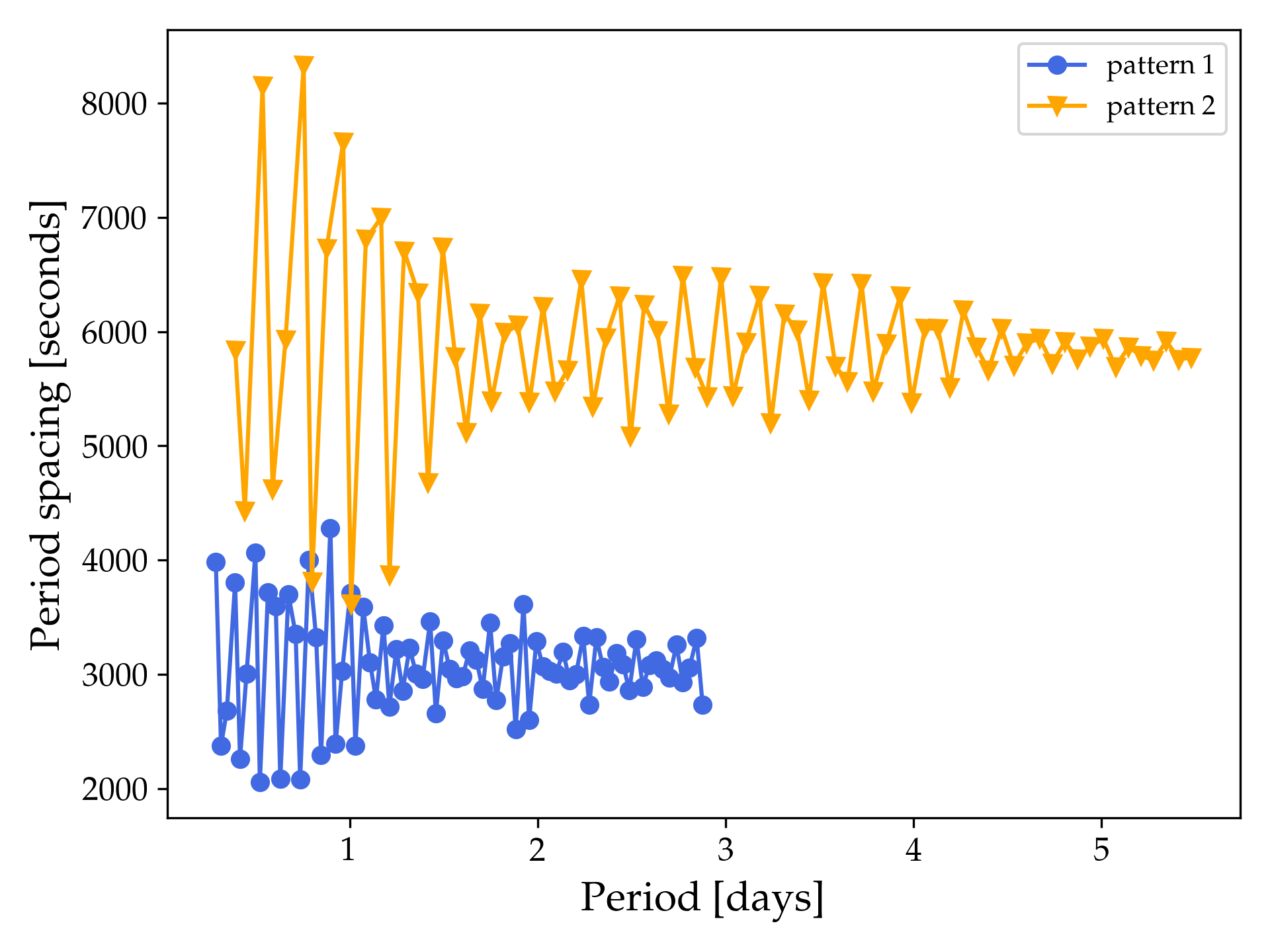
Compare the period spacing patterns for the four different overshooting parameters. How are they different/similar?
As an example of what the period spacing patterns might look like we show below the period spacing patterns calculated from the final_summary_0.01fov.txt (blue) and profile2_summary.txt (orange) GYRE output files assuming $f_{\rm ov} = 0.01$.
Bonus exercise 1: Varying GYRE input parameters
Currently, when you run GYRE you should see that all modes have $n_{\rm pg} = -n_{\rm g}$ and all g-modes between $n_{\rm g} = 3$ and $80$ are being output. The exact output will change depending on how you setup your GYRE inlist. For this bonus exercise we are going to investigate what happens when we change the parameters: freq_min, freq_max, grid_type, n_freq, and summary_item_list.
Task B1.1
Change your parameter n_freq to 10, 50, 100, 200, 400, and 600. What happens to the number of output frequencies and time it takes for GYRE to finish its calculations? What is the minimum value for n_freq that you need to get all modes from $n_{\rm g} = 5$ to $80$?
Task B1.2
Play around with the two parameters freq_min and freq_max. What values do you need to use to get the full list of ($\ell, m$) = ($1,1$) from $n_{\rm pg} = -1$ to $-80$?
Hint
You may need to increase n_freq as well.
Task B1.3
Change the parameter grid_type to 'LINEAR' then run GYRE. What happens to your output? What value do you need to use for n_freq to get the same output as before?
Task B1.4
Have a look at the possible
summary file output on the GYRE documentation website. Find the parameter for the stellar mass as well as the effective temperature perturbation amplitude and phase and included them as output for your GYRE computations. Run GYRE to make sure everything works.
Now before moving on to the next exercises, make sure you reset the parameters in your gyre.in file to the initial ones, i.e.
freq_min = 0.05
freq_max = 5.0
n_freq = 1000
grid_type = 'INVERSE'
summary_item_list = 'l,m,n_p,n_g,n_pg,freq'
Bonus exercise 2: Resolution impact on period spacing patterns
So far, aside from additional time step resolution near the end of the main-sequence evolution, we have been using the default mesh grid and time step resolution in MESA. The period spacing patterns are very sensitive to the profile of the Brunt-Vaisala frequency, as it determines where the g-modes can propagate and how they get trapped near the core as a chemical gradient is developed when the convective core contracts. Therefore, if we want to model them we have to make sure that the Brunt-Vaisala frequency profile is converged. Remember that when using MESA for any type of science, it is always important to test if your models are converged!
For this bonus exercise, we are going to play around with the two parameters mesh_delta_coeff and time_delta_coeff and see how they change the Brunt-Vaisala frequency profile.
Task B2.1
Copy profile_columns.list from $MESA_DIR/star/defaults/ to your SPB_minilab_2 work directory. Make sure that brunt_N2, brunt_N2_structure_term, and brunt_N2_composition_term are included as output.
Task B2.2
Add the following to inlist_pgstar:
Profile_Panels1_win_flag = .true.
Profile_Panels1_num_panels = 2
Profile_Panels1_yaxis_name(1) = 'brunt_N2'
Profile_Panels1_other_yaxis_name(1) = ''
Profile_Panels1_yaxis_name(2) = 'brunt_N2_structure_term'
Profile_Panels1_other_yaxis_name(2) = 'brunt_N2_composition_term'
Profile_Panels1_file_flag = .true.
Profile_Panels1_file_dir = 'png'
Profile_Panels1_file_prefix = 'profile_panels1_1.0mdc_1.0tdc_'
Profile_Panels1_file_width = 12
Profile_Panels1_file_aspect_ratio = 0.75
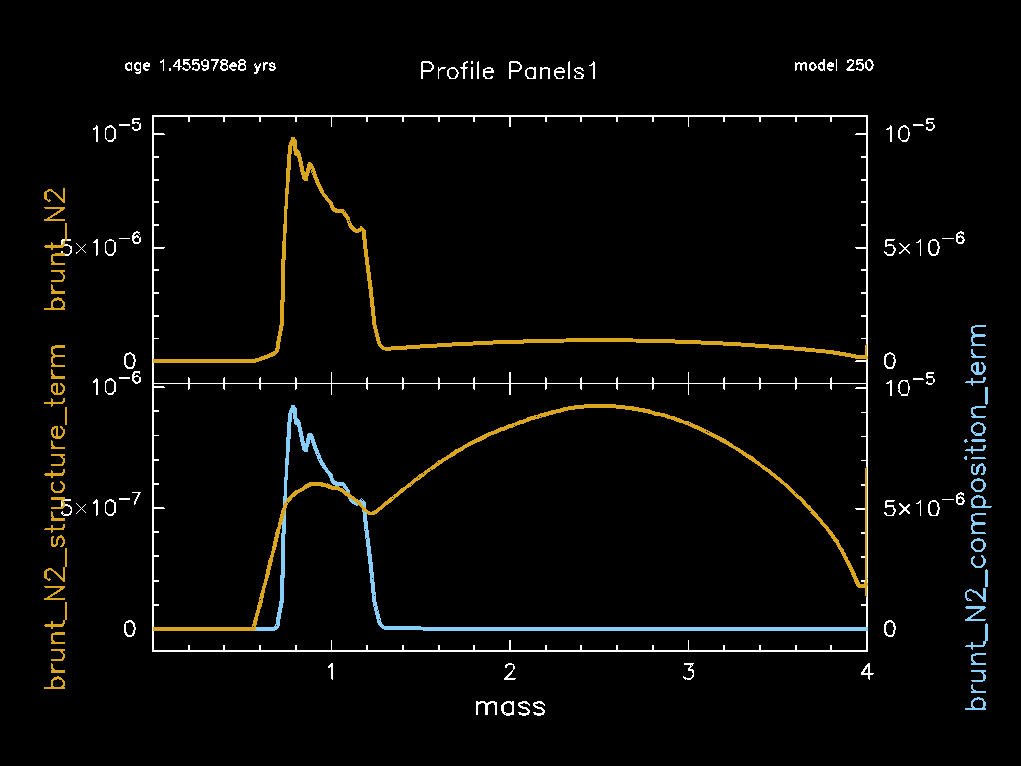
This will save the pgstar window showing the Profile_Panels1 plot to the png directory. We will need those for comparisons later. An example of what this pgstar window looks like is shown below.
Task B2.3
Include the two parameters mesh_delta_coeff = 1.0 and time_delta_coeff = 1.0 in your inlist_project under &controls. Change your output LOGS directory to log_directory = 'LOGS/4Msun_#fov_1.0mdc_1.0tdc'. Likewise make sure to change filename_for_profile_when_terminate = 'LOGS/4Msun_#fov_1.0mdc_1.0tdc/final_profile.data'. Then run MESA.
Take note of the output to the png directory. Is the Brunt-Vaisala frequency profile looking smooth?
Task B2.4
Now change the mesh_delta_coeff and time_delta_coeff parameters to match the combinations listed in the table below. Remember to also change log_directory, filename_for_profile_when_terminate, and Profile_Panels1_file_prefix accordingly to not overwrite your previous saved files. Then rerun MESA and look at how your saved profile plots of the Brunt-Vaisala frequency profile compare to each other. Do they change as you change the mesh and time resolution? If so, in what way?
mesh_delta_coeff (mdc) |
time_delta_coeff (tdc) |
|---|---|
| 1.0 | 1.0 |
| 1.0 | 0.5 |
| 0.5 | 1.0 |
| 0.5 | 0.5 |
If you also run
GYRE for each one of these configurations, you can check how the period spacing patterns are changing as well.