Introduction
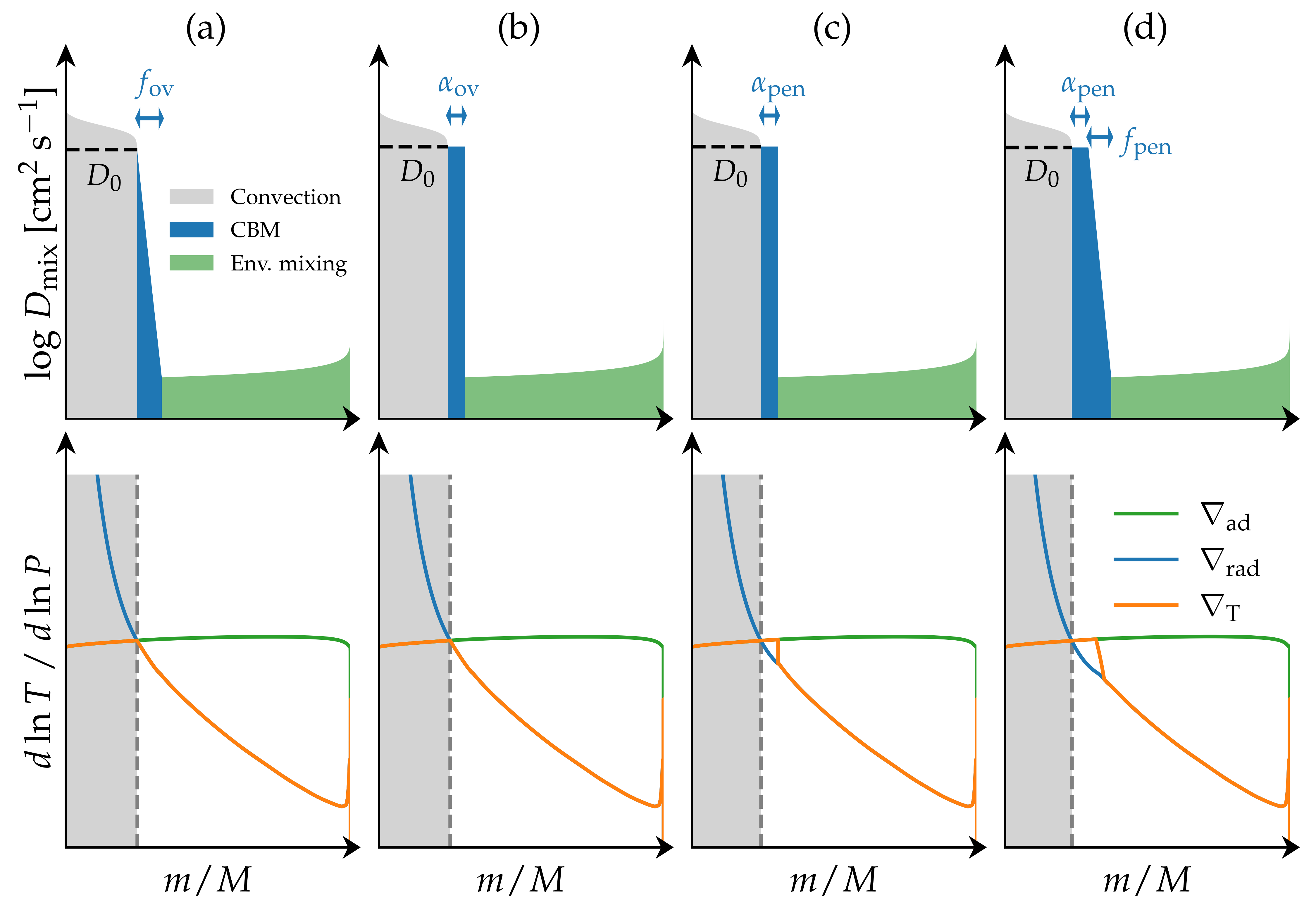
From the comparison of observations to stellar models we know that standard 1D stellar models systematically underestimate the sizes of the convective cores of intermediate- and high-mass stars. This has major consequences for the predicted evolution of the stars as larger convective core sizes translates to more fuel being available during core-hydrogen burning, leading to both longer main-sequence lifetimes and larger helium cores. One way to try to account for this is to introduce additional convective boundary mixing (CBM) beyond the Schwarzschild boundary of the convective core. Such CBM is referred to as overshooting when it only modifies the chemical structure of the star ($\nabla_{\rm T} = \nabla_{\rm rad}$), and penetrative when it modifies both the chemical and thermal structure ($\nabla_{\rm T} = \nabla_{\rm ad}$). Four examples of what such different CBM might look like are shown in the figure below. We note that in MESA “only” exponential diffusive overshooting (a) and step overshoot (b) are included as standard options.
Asteroseismology provides a powerful tool for probing not only the sizes of the CBM regions but also the shapes (Pedersen et al. 2018) of their mixing profiles as well as their thermal structure (Michielsen et al. 2019). Stars oscillating in gravity (g) modes are of particular interest, as these modes are highly sensitive to the near core regions of the stars. In these MESA labs we will focus on one such type of oscillator known as Slowly Pulsating B (SPB) stars, which are main-sequence B-type stars with masses between $3-10\,{\rm M}_\odot$ and oscillate in g-modes with periods between $0.5-5\,{\rm d}$. For a non-rotating, chemically homogeneous star the periods of the g-mode oscillations are given by
\begin{equation} P_{\ell, n} \approx \frac{\Pi_0}{\sqrt{\ell (\ell +1)}} n, \qquad \Pi_0 = 2\pi \left(\int \frac{N}{r} {\rm d}r \right)^{-1}, \end{equation}
where $\ell$ is the degree of the oscillation, $n$ is the radial order, $\Pi_0$ is the assymptotic period spacing, which we could also write as $\Pi_\ell= \Pi_0/\sqrt{\ell (\ell +1)}$, and $N$ is the Brunt-Vaisala frequency.
In this minilab we are going to take a closer look at the CBM assuming an exponential diffusive overshooting profile (panel a if the figure above), where the extent of the CBM region is determined through the free parameter $f_{\rm ov}$ (see further details below), and investigate the dependence of the main-sequence lifetimes, core masses, surface abundances, and $\Pi_\ell$ on the choice of $f_{\rm ov}$ for a $4\,{\rm M}_\odot$ SPB star.
Aims
MESA aims: In this Minilab you will learn how to look up relevant parameters to include in your MESA inlist, how to load a starting model and whether or not it cares about the initial mass and chemical composition that you use in your inlist, and how to use pgstar.
Science aims: To get an understanding of how convective boundary mixing in the form of exponential diffusive overshoot impacts the core masses (convective and helium), age, surface abundance of nitrogen, and $\Pi_\ell$, as well as the dependence of these parameters on the size of the overshooting region set by the parameter $f_{\rm ov}$.
Minilab 1
Warning! These MESA labs have been put together with both low time and spatial resolution for the sake of having the models be completed within a sensible timeframe for the summer school. Before any of these steps or result can be used in any type of actual science case, carrying out a convergence study is crucial!
Solution: In case you get stuck at any point during the exercises, then you can download the solution to minilab 1 from here. Please also note that we strongly encourage you to take advantage of the provided hints in all of the MESA labs!
In this Minilab 1, we will start constructing the inlist we need to study period spacing patterns in SPB stars and investigate the effect of convective boundary mixing on the asymptotic period spacing $\Pi_0$, the convective core mass $m_{\rm cc}$, and the helium core mass $m_{\rm He, core}$ obtained at the terminal-age main sequence (TAMS). As a first step, when starting a new project with MESA, we copy and rename the $MESA_DIR/star/work directory
cp -r $MESA_DIR/star/work SPB_minilab_1
cd SPB_minilab_1
For good measure, let’s make sure that the standard MESA inlist runs
./clean && ./mk
./rn
Let it run until the pgstar window shows up, then terminate the run using ctrl + c.
Task 1
Copy and rename the $MESA_DIR/star/work directory as demonstrated above, then compile and run MESA to check that everything is running as it should.
If everything is running as it should (if not, ask your TA for help!) then it is now time to start modifying your MESA inlists. We will be using the same inlists throughout Minilab 1, Minilab 2, and the Maxilab and keep adding things to them as we go along.
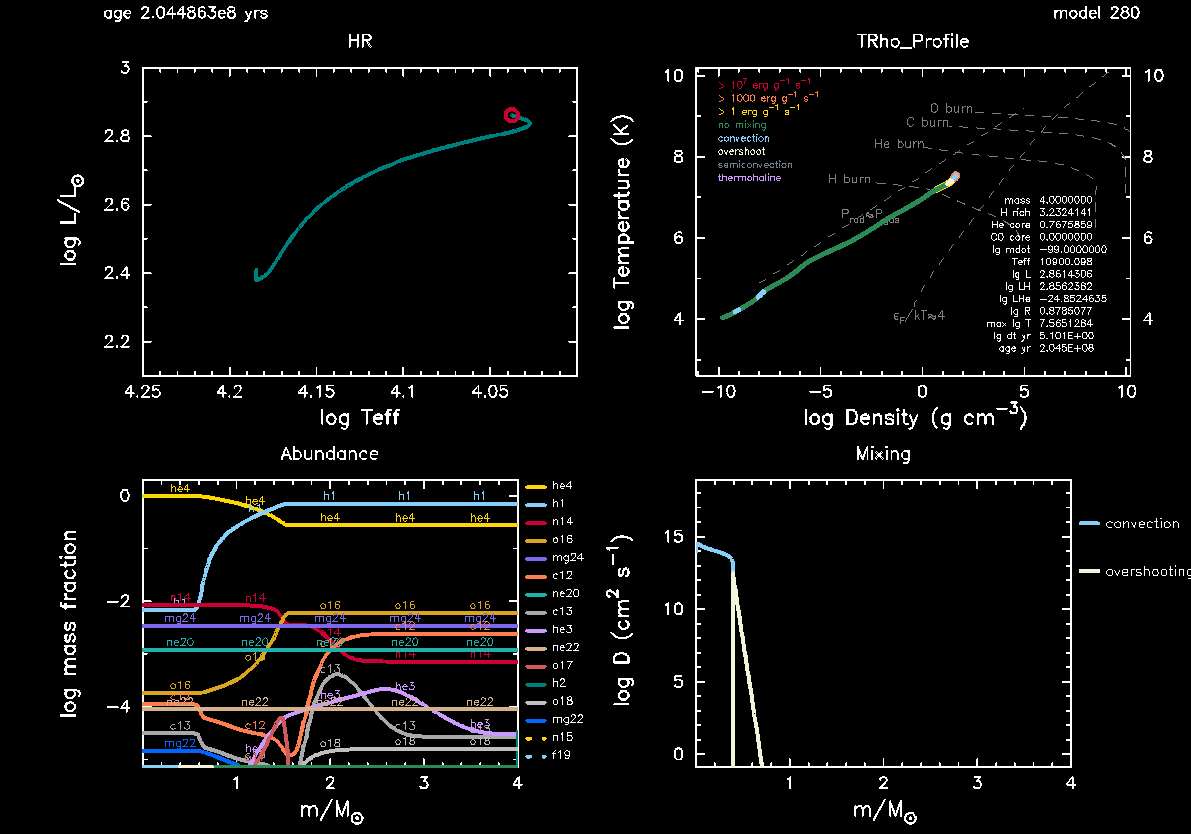
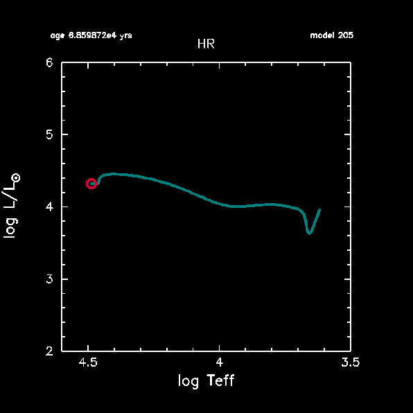
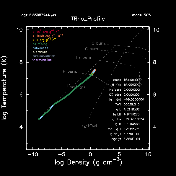
As MESA is running, you will notice that two pgstar windows show up. One is an HR diagram showing the evolutionary track of the star, with its current effective temperature and luminosity indicated by a red circle. The second window shows the current internal temperature versus density profile of the star, also indicating convective and other (non-)mixing regions by the colour of the profile, at what combined central densities and temperatures nuclear burning is taking place (part of the white dashed lines), the amount of generated energy (yellow, orange, and red outline of the profile), etc.
Both of these pgstar windows are the default windows being shown in MESA when you copy the $MESA_DIR/star/work directory. Depending on your laptop/desktop these windows might appear small and difficult to read. Fortunately, MESA provides a variety of parameters that we can use to make changes to the default pgstar windows, including their sizes. We can do so within the file inlist_pgstar. The pgstar documentation can be found here.
Task 2
Modify your inlist_pgstar file until you are satisfied with the sizes of your pgstar windows. Note that any changes that you make to inlist_pgstar and save while MESA is running are automatically updated on the fly.
Hint
The two pgstar plotting windows are called HR window
(documentation) and TRho Profile Window (documentation). The names of the parameters that you should be varying are: HR_win_width, HR_win_aspect_ratio, TRho_Profile_win_width, and TRho_Profile_win_aspect_ratio. These are already included in inlist_pgstar by default.
While we don’t recommend using figures generated with pgstar in papers, these figures are very useful both for troubleshooting and making sure that MESA is doing what we expect it to do. This will become more clear in the Maxilab once we start to include our own custom mixing profiles in MESA.
Now that the pgstar windows are on the right scale, we will focus on the inlist_project file. Usually, we want to start the evolution from the pre-main sequence, however, in an effort to save time for these labs, we will instead start the evolution at the zero-age main sequence (ZAMS) using a pre-generated starting model for a $4M_\odot$ star and evolve the star until core hydrogen exhaustion. To do this, we have to modify both &star_job and &controls.
&star_job
  ...

  ! begin with a pre-main sequence model
    create_pre_main_sequence_model = .true.
  ...

/ ! end of star_job namelist

...

&controls
  ...

  ! when to stop

    ! stop when the star nears ZAMS (Lnuc/L > 0.99)
    Lnuc_div_L_zams_limit = 0.99d0
    stop_near_zams = .true.

    ! stop when the center mass fraction of h1 drops below this limit
    xa_central_lower_limit_species(1) = 'h1'
    xa_central_lower_limit(1) = 1d-3

  ...

/ ! end of controls namelist
You can find the &star_job documentation here, while the corresponding documentation website for the &controls parameters are located here. If you want to have a look at the inlist used to create the starting model, you can look at and download it here, but you don’t need it to do these MESA labs.
Task 3
Modify the &star_job and &controls sections of inlist_project to start the evolution at the ZAMS by loading in the provided ZAMS model SPB_ZAMS_Y0.28_Z0.02.mod for a $4\,$M$_\odot$ star and stop the evolution when the core 1H mass fraction drops below 0.001. Also, include an abundance window to the pgstar output, then try to evolve the star.
Hint
The parameters that need to be changed are create_pre_main_sequence_model (&star_job) and stop_near_zams(&controls), while two additional parameters (load_saved_model and load_model_filename) have to be included in &star_job to load the SPB_ZAMS_Y0.28_Z0.02.mod file. To plot the abundance window, add Abundance_win_flag = .true. to inlist_pgstar (documentation).
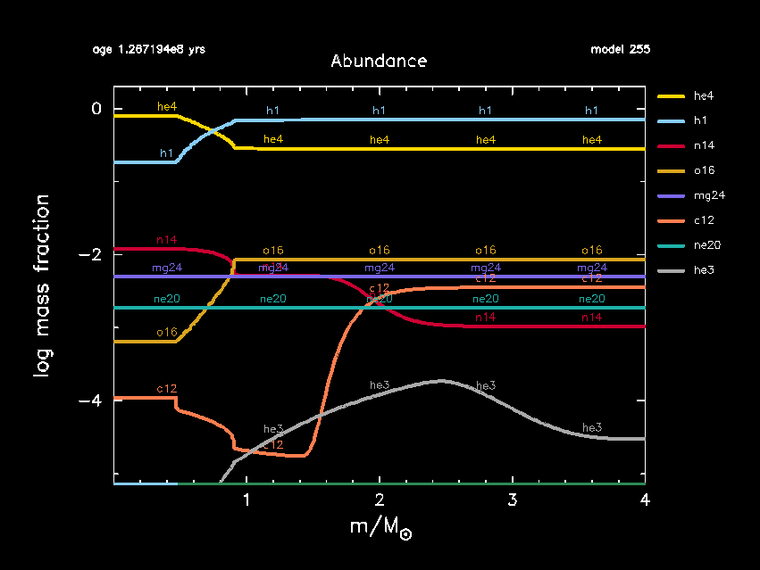
As MESA is running, you should now see a third pgstar window appear, showing the abundance profiles as a function of mass. The x-axis is color coded according to the internal mixing taking place in different regions of the star and matches that being shown in the TRho_profile window. If you are unhappy with the size of this window, you can change the size and aspect ratios of it in inlist_pgstar using the parameters Abundance_win_width and Abundance_win_aspect_ratio.
Once the main-sequence evolution is running, we will keep modifying inlist_project. First, we change the nuclear network to include additional reactions and isotopes relevant for the CNO-cycle. A list of default nuclear networks options available in MESA are listed in the $MESA_DIR/data/net_data/nets directory. We refer to the MESA labs tomorrow for more details on nuclear networks.
Task 4
What is the default nuclear network used by MESA? Change this in the &star_job section of inlist_project so pp_cno_extras_o18_ne22.net is used instead. Also include an abundance window to the pgstar output. What happens to the abundance pgstar window when you change the network?
Hint
The parameters that need to be added in inlist_project are change_net and new_net_name.
Hint
Prior to changing the network, you can find out what the name of the default nuclear network is by running MESA and looking at the terminal output. Alternatively, you can look at the parameter default_net_name in the nuclear networks controls section of the controls documentation webpage.
Next, we are going to change the name of the LOGS directory where the MESA output history.data and profile#.data files get saved in preparation for varying the convective boundary mixing of the star without overwriting previous MESA calculations. We will also relax the composition of the star to match the Galactic standard measured from B-type stars in the solar neighbourhood (Nieva & Przybilla 2012; Przybilla et al. 2013), change the opacity tables to the OP tables calculate for the metal mixture of Asplund et al. (2009) to match the initial metal mixture used in our starting model SPB_ZAMS_Y0.28_Z0.02.mod for the sake of consistency, and increase the frequency at which the history output is saved to the history.data file.
The choice of opacity tables and metal mixtures is particularly important when we try to predict which oscillations get excited by the $\kappa$-mechanism (i.e. opacity or heat mechanism), which depending on the type of pulsating star operates in the partial ionization zones of hydrogen, helium, or iron-group elements. In the case of SPB stars, the g-mode oscillations are excited by the $\kappa$-mechanism operating in the partial ionization zone of the iron-group elements, also known as the iron opacity bump or $Z$ bump. The choice of the metal mixture determines how the mass fractions of the metal isotopes (i.e. anything other than hydrogen and helium) are distributed, and highly impacts the opacities in the iron bump as demonstrated in the figure below.
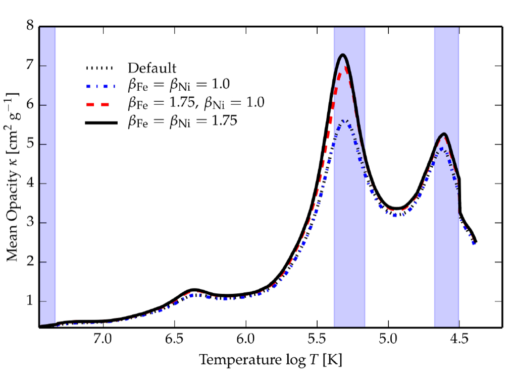
MESA opacity profile is shown in dashed blue. Corresponding opacity profiles resulting from increasing the opacity contribution of iron (red dashed) and both iron and nickel (full black) to the Rosseland mean opacity by 75% clearly show an increase in the opacity in the partial ionization zone of iron-group elements at around $\log T\sim 5.3$. Credit: Morraveji (2016).The choice of opacities and metal mixtures will also modify the predicted oscillation frequencies (see, e.g., Figure 3 of Morraveji et al. (2015)). While new metal mixtures closer to the ones by Grevesse & Sauval (1998) than Asplund et al. (2009) have recently been found by Magg et al. (2022), the corresponding opacities in the Z-bump derived for the Grevesse & Sauval (1998) metal mixture are lower than those using Asplund et al. (2009). Given the general need for higher opacities in the Z-bump from nickel required to explain the number of excited modes in both $\beta$ Cep and SPB stars (e.g. Walczak et al. (2019) and Szewczuk et al. (2022)), the metal mixture of Asplund et al. (2009) is used in these MESA lab exercises.
More detailed studies of mode excitation are outside the scope of these MESA labs and we refer instead to previous MESA labs by Rich Townsend and Radek Smolec from the 2019 and 2021 MESA Summer Schools.
Task 5
Make the following additional changes to inlist_project. The text in the parenthesis indicates where in the inlist_project file the required changes have to be made.
- Change the output LOGS directory to
LOGS/4Msun_0fov(&controls). - Relax the composition to $X=0.71$, $Y=0.276$, and $Z=0.014$ (
&star_job,&kap, and&controls). In&controlsadd the following two parameters:relax_dY = 0.001andrelax_dlnZ = 1d-2. These latter two parameters determine how quickly the composition is relaxed to the new desired values of $Y$ and $Z$. - Use the OP opacity tables for the Asplund et al. (2009) metal mixture (
&kap) and make sure also to set theZbaseparameter (&kap, documentation) equal to 0.014 so the base metallicity of the opacity tables match the new value of $Z$. - Set
pgstarto pause before terminating (&star_job). - Output history data at every time step instead of every fifth time step (
&controls).
Hint
The parameters that need to be added in &star_job are: relax_Y, new_Y, relax_Z, new_Z, and pause_before_terminate.
Hint
The parameters that need to be added in &controls are: log_directory, relax_dY = 0.001, relax_dlnZ = 1d-2, and history_interval.
Hint
Concerning figuring out how to set the kap_file_prefix parameter, you might notice if you look up this parameter on the MESA documentation website that the following options are listed: gn93, gs98, a09, OP_gs98, and OP_a09_nans_removed_by_hand. However, no explanation is given as to what these parameters actually stand for. From the naming of the parameters you might be able to guess which one you have to use, but if you want to be sure then one way to do this is to go to your $MESA_DIR/data/kap_data/ directory and look at the files there. In the file names, everything before _z#.#_x#.#.data corresponds to the input options for the kap_file_prefix parameter. If you choose one of the files there and open it, then the first line of the file will give you the explanation and reference to the table.
If in doubt, your inlist_project should now look something like this.
Once you have implemented the changes above, delete the contents of your current LOGS directory. Then try to run MESA and see if all the implemented changes work as they should. If you tried to change the two parameters initial_z and initial_y to match the new compositions, you would see in the terminal output that MESA is ignoring these changes. You may also see that although the parameter initial_mass = 15 is still set in the inlist_project file, then this choice of initial mass is also being ignored. As a reminder, the mass of the loaded model is $4M_\odot$.
 ___________  ...  ___________   ...	_________ ...

       step   ...  Mass          ...	Y_surf    ...
  lg_dt_yrs   ...  lg_Mdot       ...	Z_surf    ...
    age_yrs   ...  lg_Dsurf      ...	Z_cntr    ...
 ___________  ...  ___________   ...	_________ ...

        240   ...  4.000000      ...	0.280000  ...
 6.3041E+00   ...  -99.000000    ...	0.020000  ...
 1.0143E+08   ...  -9.311364     ...	0.019646  ...
This is because the initial mass and composition have already been set by the input MESA model SPB_ZAMS_Y0.28_Z0.02.mod, which we are telling MESA to load. If we wanted to change these values, then we can relax the composition of the input model (as we are doing in this minilab) and likewise, we can relax the initial mass of the model.
Once your new inlist_project is working, the next step is to start including convective boundary mixing. Before doing so, lets adjust the plotting window of the pgstar HR diagram and include one additional pgstar plotting window showing the mixing profile. You may also notice that the evolutionary track showing up in the HR window only takes up a small part of the pgstar plot. This is because we are now considering a $4M_\odot$ star instead of the default $15M_\odot$ star, and we are focusing only on the main-sequence evolution. An example comparison of the HR window before and after zooming in on the evolutionary track is shown below.
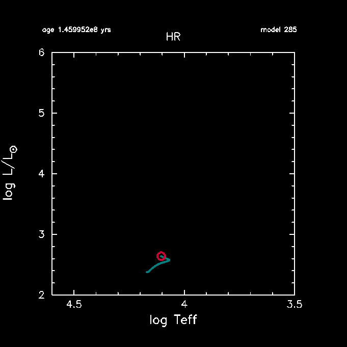
HR window before modifying x- and y-axes limits.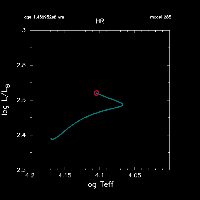
HR window after modifying x- and y-axes limits.Task 6
Zoom in on the MS evolutionary track of the start in the pgstar HR window and include an additional pgstar window showing the mixing profile.
Hint
Modify the four input parameters HR_logT_min, HR_logT_max, HR_logL_min, and HR_logL_max in inlist_pgstar. You can do this on the fly while MESA is running. Look up "Mixing window" in the MESA pgstar documentation. The parameter you want to add to inlist_pgstar is Mixing_win_flag.
If in doubt, your inlist_pgstar should look something like this.
The final input parameters we want to add to inlist_project are related to the convective boundary mixing. For this exercise, we will only consider exponential diffusive overshoot on top of the hydrogen-burning convective core:
This type of mixing is one out of two overshoot mixing schemes that have been implemented in MESA. $D_0$ is the diffusive mixing coefficient at $r_0 = r_{\rm cc} - f_0 H_{\rm p,cc}$ , i.e. at a step of $f_0 H_{\rm p,cc}$ inside the convective core boundary at radius coordinate $r_{\rm cc}$. This step is required because the diffusive mixing coefficient for the convective zone approaches zero at the core boundary. $H_{\rm p,0}$ is the pressure scale height at $r_0$, $H_{\rm p, cc}$ is the pressure scale height at $r_{\rm cc}$, $f_{\rm ov}$ is the overshoot parameter, and $f_0$ is a numerical parameter which is typically fixed at a value smaller than $f_{\rm ov}$. For this exercise, we will fix $f_0 = 0.002$ and vary $f_{\rm ov}$ from 0.005 to 0.04.
Task 7
Look up the parameters required to include convective boundary mixing (overshoot) in MESA. Include these parameters in inlist_project (&controls), replace the (:) with (1), set the overshoot scheme to exponential on top of the core during hydrogen burning, set $f_0 = 0.002$, and choose a value for $f_{\rm ov}$ between 0.005 to 0.04. Run MESA. Change the name of your output LOGS directory LOGS/4Msun_#fov so that # corresponds to your choice of $f_{\rm ov}$. What happens to the pgstar mixing and HR windows? Note that models with a higher $f_{\rm ov}$ parameter will take longer to run, so if your laptop is slow make sure to choose a low value and have someone else at your table choose a high value.
Hint
The parameters to be added to &controls in inlist_project are: overshoot_scheme(1), overshoot_zone_type(1), overshoot_zone_loc(1), overshoot_bdy_loc(1), overshoot_f(1), and overshoot_f0(1) = 0.002. overshoot_f(1) is the overshooting parameter that you will be varying.
Task 8
Include overshoot_D_min = 1d-2 in inlist_project (&controls). What happens to the mixing profile shown in your mixing window? What is the default value of overshoot_D_min?
(If in doubt, your inlist_project should now look something like this.)
Your final pgstar mixing window should end up looking something like this depending on your choice of $f_{\rm ov}$:
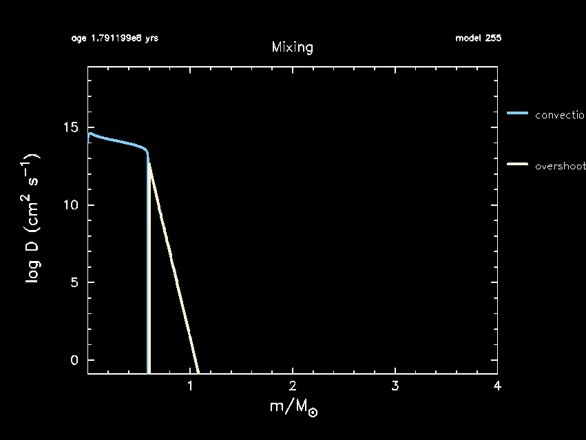
Now that we have the desired physics included in our MESA inlists, it is time to see how exponential diffusive overshooting impacts the convective core mass ($m_{\rm cc}$), the helium core mass obtained that the TAMS ($m_{\rm He, core}$), the age of the star at the TAMS ($\tau_{\rm TAMS}$), the 14N mass fraction at the surface X(14N)surf, and the asymptotic period spacing of $\ell =1$ g-modes ($\Pi_{\ell=1}$). To do so, we first have to make sure that these are included as part of the history output.
Task 9
Copy history_columns.list from $MESA_DIR/star/defaults to SPB_minilab_1. Make sure that the following parameters are included in history_columns.list: mass_conv_core, he_core_mass, surface n14, center h1,
and delta_Pg. Also add the parameter delta_Pg_mode_freq = 20 (see details below) to your inlist_project file under &controls.
Run MESA and answer/do the following:
- In the Google spreadsheet note down your name and choice of $f_{\rm ov}$, as well as $m_{\rm He, core}$, $\tau_{\rm TAMS}$, and $X(^{14}{\rm N})_{\rm surf}$ at TAMS.
- Find the value of $\Pi_{\ell=1}$ and $m_{\rm cc}$ at
center_h1 ∼ 0.35(i.e. halfway through core hydrogen burning) and add these to the Google spreadsheet. - How do these values change for different values of $f_{\rm ov}$?
delta_Pg_mode_freq clarification
The asymptotic period spacing is given by the integral over the region in which a g-mode can propagate.
Hence you need a specific mode frequency in mind when you do this calculation, because above a certain radius, your
mode frequency is much larger than both the Brunt-Vaisala and Lamb frequencies and hence your g-mode is evanescent there.
This delta_Pg_mode_freq allows you to pick a frequency which in turn will determine the integration limits.
Note that if you want to use asymptotic period spacing values in a scientific publication, you might want to write some functionality in the run_star_extras.f90 to calculate the values yourself instead.
Hint
The convective core mass (mass_conv_core), helium core mass (he_core_mass), star age (star_age), and center 1H mass fraction (center_h1) parameters are already included in the history output by default. The only additional ones you have to add are surface n14 and delta_Pg. Note that the formatting for adding center and surface abundances inside the history_columns.list file is center n14 and surface n14, but shows up as center_n14 and surface_n14 in your history.data file.
Hint
When finding the values at center_h1 ∼ 0.35 just select the ones that are closest to this value.
Bonus exercise: Combining multiple pgstar plots in one window
Currently, when running MESA you have four pgstar windows open at once. This is starting to get a bit busy. MESA actually has options for including multiple pgstar plots in the same window! For this bonus exercise, we will do just that. To get our (currently) four pgstar windows into one window, we’ll make use of a so-called grid. You can activate a total of nine such grids, and each grid can contain multiple plots. Today, we’ll only use one grid.
Task B1
Add the relevant inlist settings to inlist_pgstar to create a grid with 2 rows, 2 columns and 4 plots. Don't worry about trying to include your individual pgstar plots in the grid just yet. Also, make sure to include the two parameters log_center_T and log_center_Rho in your history_columns.list file, otherwise MESA will give an error right after relaxing the composition. Then run MESA.
Hint
You'll find the relevant settings under the Grid section of the pgstar documentation.
When running the model, you’ll see a fifth pgstar window appear, in which the central $T\text{–}\rho$ evolution is shown again. We obviously want to get rid of the individual windows first and then start filling our grid.
Task B2
Disable the individual pgstar windows. Afterwards, add them to the grid instead. You can do this using the Grid1_plot_name(:) array by replacing the : with 1, 2, 3 and 4, respectively. Do not remove the other inlist settings such as HR_logT_min and show_TRho_Profile_legend = .true.. They will still apply to our plots, even though they live in the grid now.
Hint
The names required to add the desired plots to the grid are the same as those used for the individual pgstar windows. For example: to add the $T\text{-}\rho$-profile (previously enabled by TRho_Profile_win_flag = .true.), the name should be TRho_profile.
What we want to do next, before running our model again, is assign each of our four plots to a location on the grid. We can do this by specifying the row and column number. We also want to make sure each plot only takes up the width and height of one column and row, respectively.
Task B3
Find the inlist settings to assign each plot (HR, TRho_profile, Abundance and Mixing) to a location in the grid, and make sure they only span one column width and row height. You can choose for yourself where in the grid you want which plot. After you've done this, run the model again.
Hint
Just as for the Grid1_plot_name(:), the row(span)/column(span) settings are handled by an array.
Hint
The row/column indices in our $2\times 2$ grid are $[1,\,2]$.
If you’ve run the model, chances are that the pgstar window looks quite horrible now, with overlapping plots etc. To make the window prettier, we’re going to have to play with some of the window dimensions, individual plot padding, and scaling settings. Now for some good news and some bad news. The bad news is that these settings depend on what kind of screen you’re working on. The specific settings in the solution below work for the laptop of the person writing this, but not necessarily for yours. The good news is that you can adjust the inlist settings during the run. Simply saving inlist_pgstar will apply your settings to the pgstar window while MESA is running.
Task B4
Adjust the settings for the grid window dimensions, padding for the individual plots, and text scale factors to make each plot fit nicely in the pgstar window. Run the model until you're satisfied with how the pgstar window is looking.
Hint
The pgstar parameters you need to add and vary are:
Grid1_win_widthGrid1_win_aspect_ratioGrid1_plot_pad_left(:)Grid1_plot_pad_right(:)Grid1_plot_pad_top(:)Grid1_plot_pad_bot(:)Grid1_txt_scale_factor(:)
If all went well, your inlist_pgstar should look something like the one below. In the next labs, you will need to add additional pgstar plots. If you have time left, you can always try to add them to the grid you just made!
&pgstar

! Grid window settings
  Grid1_win_flag = .true.
  Grid1_win_width = 18
  Grid1_win_aspect_ratio = 0.65
  Grid1_num_cols = 2
  Grid1_num_rows = 2
  Grid1_num_plots = 4

! HRD
  Grid1_plot_name(1) = 'HR'
  Grid1_plot_row(1) = 1
  Grid1_plot_rowspan(1) = 1
  Grid1_plot_col(1) = 1
  Grid1_plot_colspan(1) = 1
  Grid1_plot_pad_left(1) = 0.0
  Grid1_plot_pad_right(1) = 0.05
  Grid1_plot_pad_top(1) = 0.0
  Grid1_plot_pad_bot(1) = 0.05
  Grid1_txt_scale_factor(1) = 0.7
  HR_logT_min = 4.0
  HR_logT_max = 4.25
  HR_logL_min = 2.1
  HR_logL_max = 3.0

! Temperature-density profile
  Grid1_plot_name(2) = 'TRho_profile'
  Grid1_plot_row(2) = 1
  Grid1_plot_rowspan(2) = 1
  Grid1_plot_col(2) = 2
  Grid1_plot_colspan(2) = 1
  Grid1_plot_pad_left(2) = 0.05
  Grid1_plot_pad_right(2) = 0.0
  Grid1_plot_pad_top(2) = 0.0
  Grid1_plot_pad_bot(2) = 0.05
  Grid1_txt_scale_factor(2) = 0.7
  show_TRho_Profile_legend = .true.
  show_TRho_Profile_text_info = .true.

! Abundances
  Grid1_plot_name(3) = 'Abundance'
  Grid1_plot_row(3) = 2
  Grid1_plot_rowspan(3) = 1
  Grid1_plot_col(3) = 1
  Grid1_plot_colspan(3) = 1
  Grid1_plot_pad_left(3) = 0.0
  Grid1_plot_pad_right(3) = 0.1
  Grid1_plot_pad_top(3) = 0.075
  Grid1_plot_pad_bot(3) = 0.0
  Grid1_txt_scale_factor(3) = 0.7

! Mixing
  Grid1_plot_name(4) = 'Mixing'
  Grid1_plot_row(4) = 2
  Grid1_plot_rowspan(4) = 1
  Grid1_plot_col(4) = 2
  Grid1_plot_colspan(4) = 1
  Grid1_plot_pad_left(4) = 0.05
  Grid1_plot_pad_right(4) = 0.05
  Grid1_plot_pad_top(4) = 0.075
  Grid1_plot_pad_bot(4) = 0.0
  Grid1_txt_scale_factor(4) = 0.7

/ ! end of pgstar namelist
The corresponding pgstar grid window should look something like this.